Live plotting

Note

The live plotting functionality is part of blocks-extras, which must be separately installed.

Plots often give a clearer image of your training progress than textual logs. This is why Blocks has a Plot extension which allows you to plot the entries from the log that you are interested in.

We use Bokeh, an interactive visualization library, to perform the plotting. More specifically, we use the Bokeh Plot Server. This is basically a light web server to which Blocks can send data, which then gets displayed in live plots in your browser. The advantage of this approach is that you can even monitor your models’ training progress over a network.

First, make sure that you installed the necessary requirements (see the installation instructions). To start the server type

$ bokeh-server

This will start a server that is accesible on your computer at http://localhost:5006. If you want to make sure that you can access your plots across a network (or the internet), you can listen on all IP addresses using

$ bokeh-server --ip 0.0.0.0

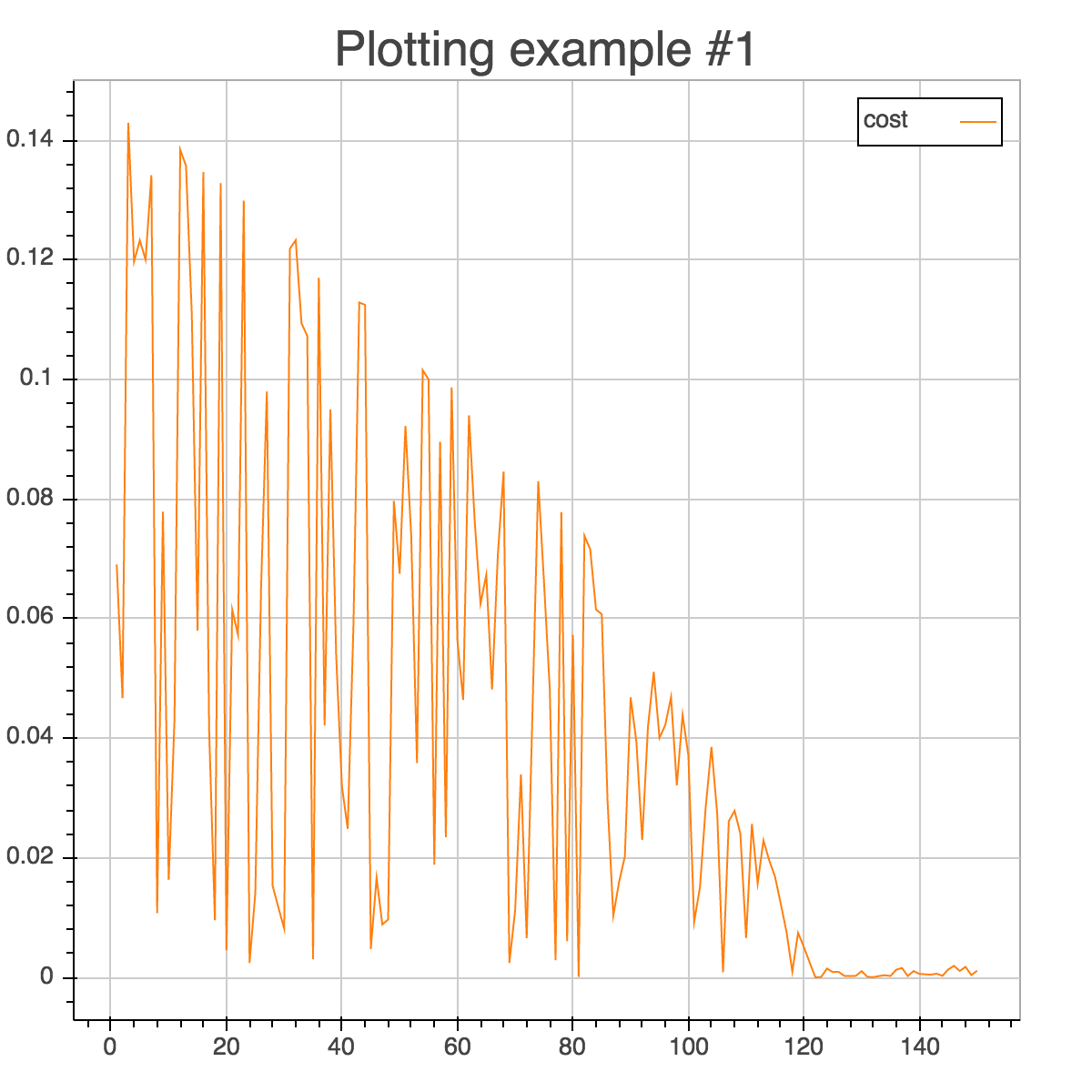
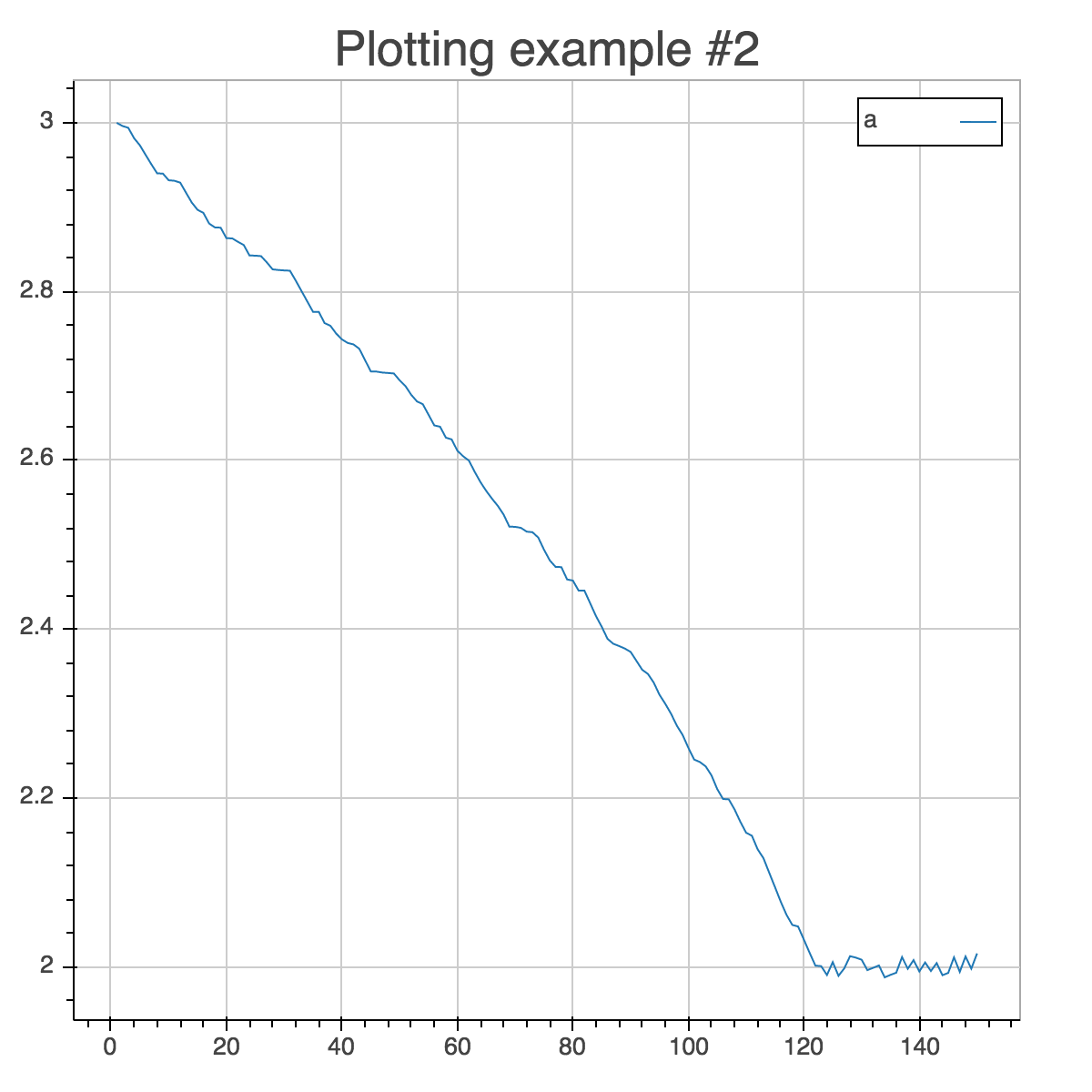
Now that your plotting server is up and running, start your main loop and pass the Plot extension. Consider this example of fitting the function \(f(x) = x^a\) to \(f(x) = x^2\).

>>> import theano
>>> a = theano.shared(3.)
>>> a.name = 'a'
>>> x = theano.tensor.scalar('data')
>>> cost = abs(x ** 2 - x ** a)
>>> cost.name = 'cost'

We train on a 150 random points in \([0, 1]\).

>>> import numpy
>>> from fuel.streams import DataStream
>>> from fuel.datasets import IterableDataset
>>> data_stream = DataStream(IterableDataset(
...     numpy.random.rand(150).astype(theano.config.floatX)))

Now let’s train with gradient descent and plot the results.

>>> from blocks.main_loop import MainLoop
>>> from blocks.algorithms import GradientDescent, Scale
>>> from blocks.extensions import FinishAfter
>>> from blocks.extensions.monitoring import TrainingDataMonitoring
>>> from blocks.extras.extensions.plot import Plot  
>>> main_loop = MainLoop(
...     model=None, data_stream=data_stream,
...     algorithm=GradientDescent(cost=cost,
...                               parameters=[a],
...                               step_rule=Scale(learning_rate=0.1)),
...     extensions=[FinishAfter(after_n_epochs=1),
...                 TrainingDataMonitoring([cost, a], after_batch=True),
...                 Plot('Plotting example', channels=[['cost'], ['a']],
...                      after_batch=True)])  
>>> main_loop.run() 

Tip

If you want to plot channels in the same figure, pass them as part of the same list. For example, [['cost', 'a']] would have plotted a single figure with both the cost and the estimate of the exponent.

Open up your browser and go to http://localhost:5006 to see your model cost go down in real-time!